Simulation of urban microclimate with uhiSolver: software validation using simplified material data

Abstract

Background

Increasing urbanization as well as global warming requires an investigation of the influence of different construction methods and ground surfaces on the urban heat island effect (UHI effect). The extent of the influence of the urban structure, the building materials used and their surfaces on the UHI effect can be significantly reduced already in the planning phase using a designated OpenFOAM-based solver “uhiSolver”.

Results

In the first part of this research work, it is shown that inner building details and components can be neglected while still obtaining sufficiently accurate results. For this purpose, the building model was divided into two layers: a surface layer without mass, where the interaction with radiation takes place, and a component layer, which contains all relevant components and cavities of the building represented with mass-averaged material properties. It has become apparent that the three parameters—albedo, heat capacity and thermal resistance—which have a decisive influence on the interaction, have different effects on the component temperatures and the surface temperatures. In the second part of this research work, dynamic 3D computational fluid dynamics (CFD) simulations are performed with uhiSolver for a residential block in Vienna. Comparing the simulation results with measurement data collected on site, it is shown that the simplified assumption of homogeneous material data for building bodies provides very good results for the validation case investigated. However, the influence of the greening measures in the courtyard of the residential block on the air temperature is found to be negligible. Furthermore, it was observed that due to locally higher radiation density, lower air velocities and higher air humidity, the apparent temperature in the courtyard is sometimes perceived to be higher than in the adjacent streets, despite the lower air temperature.

Conclusions

Simplifying the modeling process of the uhiSolver software by reducing the model complexity helps to reduce manual work for setting up appropriate boundary conditions of buildings. Compared to market competitors, good results are obtained for the validation case Kandlgasse presented in this research work, despite the simplifications proposed. Thus, uhiSolver can be used as a robust analytical tool for urban planning.

Introduction

Background

Over the past 40 years, the temperature in Austria has risen significantly during the summer months. The seasonal increase in temperature during this period is about 2 °C (Zentralanstalt für Meteorologie und Geodynamik 2002). Especially in cities, the issue of heat stress is becoming increasingly important. The decisive factor for the heat stress is the lower night-time cooling of urban areas compared to the rural environment. During the day, the difference in temperature between the city and the surrounding area is generally up to 1 °C, whereas at night it can exceed 5 °C (Schmid and Pröll 2020). During a heat wave in August 2015, a night-time air temperature of up to 25 °C was measured in the city center of Vienna, which is about seven degrees above the average night-time air temperature of the years 1971–2000 (Zentralanstalt für Meteorologie und Geodynamik 2002). At such high night-time temperatures, living spaces can no longer be cooled down sufficiently by natural ventilation and the human organism is unable to recover from the heat stress during the day (Schmid and Pröll 2020).

Urban heat islands are of great global importance because today more people live in urban than in rural areas already. This number will continue to rise—according to predictions, two-thirds of the world population will live in cities by 2050 (United Nations Department of Economic and Social Affairs 2018). Climatically driven urban planning is essential to keep overheating of cities to a minimum (Schmid and Pröll 2020). The urban heat island effect can be reduced not only by careful planning of the urban structure, but also by a well-considered use of building materials and surfaces. Greening measures on the building scale (e.g., green walls and roofs) can have a decisive effect in terms of urban heat mitigation, which was shown in several research studies already (Mursch-Radlgruber et al. 2009; Technische Universität Wien and Universität für Bodenkultur Wien 2018; Korjenic et al. 2018, 2020; Hollands et al. 2018; Mitterböck and Korjenic 2017). In most construction projects, however, the effects on the microclimate are not yet taken into account, since often both the planners and the construction companies lack an understanding of this topic. Numerical simulation models using computational fluid dynamics (CFD) simulations can help to understand the complex interactions between the building structure and the microclimate and thus create the basis for mitigating urban heat island effects (Toparlar et al. 2015).

To avoid thermal stress caused by urban heat islands, it is important to take into account all relevant factors in the assessment of thermal comfort. The four environmental factors are air temperature, humidity, air flow and radiation. The personal factors are the clothing and the level of physical activity (B. of M. Commonwealth of Australia 2010). There are many methods of combining these factors into a single number to assess the outdoor thermal environment—for example, the Wet Bulb Globe Temperature (WBGT) (B. of M. Commonwealth of Australia 2010), the Universal Thermal Climate Index (UTCI) (Jendritzky et al. 2001), the Physiologically Equivalent Temperature (PET) (Honjo 2009) as well as the Apparent Temperature (AT) (Steadman 1994). Another way to assess thermal comfort is to calculate the thermal comfort indices Predicted Mean Vote (PMV) and Predicted Percentage of Dissatisfied (PPD), using the Fanger’s method proposed in ISO Standard 7730 (Gameiro da Silva 2013), or the Human Thermal Model (HTM) which can be used for predicting thermal behavior of the human body under both steady-state and transient indoor environment conditions (Holopainen 2012).

Within the validation case investigated in this study the apparent temperature is used for the assessment of thermal comfort, being a well-documented and relatively robust standard for subjective, felt temperature. It is determined by the simulation program uhiSolver, which is described in detail in the following section.

Numerical models in microclimate modeling

There are several numerical models in microclimate modeling at different spatial scales available nowadays, ranging from the meteorological mesoscale (< 200 km) over the meteorological microscale (< 2 km) to the building scale (< 100 m) and the indoor environment (< 10 m) (Toparlar et al. 2017). Some exemplary numerical models at the meteorological microscale are ENVI-met, Ladybug, Urban Weather Generator (UWG) and ANSYS (ENVI_MET Decoding urban nature. https://www.envi-met.com/de/; Ladybug. https://www.ladybug.tools/ladybug.html; Urban Weather Generator 4.1 urban heat island effect modeling software. http://urbanmicroclimate.scripts.mit.edu/uwg.php; Ansys. https://www.ansys.com/). In Austria, the application of the Greenpass Editor is widely used, which is based on a microclimate simulation with the ENVI-met software (GREENPASS Software http://envi-met.info/). The three-dimensional microclimate simulation model ENVI-met is used in the fields of climatology, urban planning, architecture and construction. It is designed for microscale simulations with a horizontal resolution from 0.5 m to 10 m and a time frame of 24–48 h with a time step of 1–5 s. This resolution allows to analyze small-scale interactions between individual buildings, surfaces and plants (ENVI-met Model Architecture 2019). The physical properties of the wall or façade that are considered in the model are reflectivity, absorption, transmittance, emissivity, thermal conductivity, specific heat storage capacity and the thickness of the wall. Heat flows parallel to the surface of the building component are not taken into account (Huttner and Bruse 2009). In the latest release of ENVI-met up to 3 different materials can be assigned to a wall structure (ENVI-met Model Architecture 2019; Terjung and O’Rourke 1980).

The calculation method allows a rough estimate of the energy balance and thus the temperature within individual buildings. For this calculation, the buildings are considered as empty air volumes. Neither the heat storage capacity of elements in the building nor the internal heat flows are taken into account. In order to enable the comparability of the simulation results with measured data, the daily variations of the atmospheric boundary conditions (main wind flow, temperature, humidity and air turbulence) as well as the incoming radiation can be defined (Huttner and Bruse 2009).

Another microclimate simulation program currently under development is the so-called uhiSolver from Rheologic GmbH in Vienna. As part of the “UHI Black Box” research project funded by the FFG (Austrian Research Promotion Agency), the technical feasibility of a “black box model” was tested between May 2019 and April 2020 in order to implement different building types and ground surfaces in the uhiSolver software. The manual effort of model creation was to be minimized by reducing the parameter diversity without significantly influencing the accuracy of the simulation with regard to the results for the assessment of the urban microclimate.

uhiSolver is a microclimate simulation program based on the OpenFOAM library. It combines compressible fluid flow (of air), buoyancy effects due to air density, heat conduction in solids (within buildings and ground), radiation and sun’s movement across the sky, shadows from buildings and vegetation, air flow modulation through zones of vegetation and evapotranspiration in one program. In the same way as ENVI-met and ANSYS, uhiSolver uses a fully coupled approach, i.e., the building volume interacts with radiative heat transfer (incoming and outgoing), thermal conduction (incoming and outgoing) and advective heat transfer with the surrounding airflow.

Compared to market competitors (like ENVI-met, ANSYS, etc.) uhiSolver has a few advantages:

• solid code base with long history and an open/international review process and regular core code updates;

• higher accuracy of fluid flow close to buildings, ground and any architectural details compared to voxelized simulation methods due to finite volume method and arbitrarily shaped polyhedral finite volume cells;

• support for general building shapes and modern architecture like 3D curved walls and roofs, thoroughfares;

• building details smaller than 0.5 m can be included, with spatial precision in the range of centimeters;

• validated evaporation modeling (FFG IS5k, Final report, Nr. 849231, project ‘vmSol’, Rheologic GmbH and TU Vienna, 20.10.2015, internal communication) (evaporation from wet surfaces and condensation on smooth surfaces);

• the forced inlet conditions can be modeled after actual historic meteorological data from the simulated site—e.g., inlet air temperature, humidity, etc., can change minute-by-minute;

• highly scalable software running from workstation to many/multi-core systems and high-performance computer clusters;

• achieves real-time simulation speed for urban microclimate cases.

The models shown in Fig. 1 are for the most part a combination of standard CFD models for flow and radiation that have been extensively covered in literature (see Coelho et al. 1998; Knaus et al. 1999; Ismail and Salinas 2004; Pecka 2014; Cid and Vianna 2016; Sá da Costa 2016; Mould 2019). Solar radiation, for example, is implemented using the finite volume Discrete Ordinates Method (fvDOM). Absorption through vegetation (shading) is modeled using multi-band absorptivity and emissivity coefficients, i.e., “optical” leaf density.

Fig. 1

Rheologic uhiSolver model structure

Geometry basis is a combination of publicly available 3D data and manual building modeling. Gables are included in the building models. uhiSolver can read all 3D geometries the OpenFOAM library is capable of but has no own 3D modeler included. 3D modeling is done with external programs and importing geometry from common, industrial software for architecture is supported. The spatial simulation resolution is not uniform across the simulated volume; it is higher closer to the buildings (in the order of 0.3 m at the building surface) and lower further away from the buildings.

Scope of study

The study aims to simplify the modeling process of the above mentioned uhiSolver software. The main reason for the reduction of model complexity, i.e., level of inner detail for buildings, is to reduce manual work for setting up appropriate boundary conditions of buildings. For higher levels of internal detail each and every façade and roof would have to be treated differently because of its differing thermal coefficients, leading to an unfeasible and thus uneconomic complexity and amount of manual work in setting up large scale simulations. Although this is possible using the simulation software and it is not limited by algorithmic or modeling restrictions, the greatest parts of manual set-up work and program interaction were reduced to prioritize automation, scalability and ease of variability of input data over possible higher local modeling accuracy. The development and practical application of uhiSolver are therefore driven not only by scientific insights, but also by stringent economic considerations.

For better reading, this research work is divided into two parts, the first part (Sect. “Generation of simplified material data”) including the elaboration of the simplified material data using a fictitious model building, whereas the second part (Sect. “Validation case Kandlgasse”) covers the validation on an actual residential block in Vienna. Furthermore, a recent larger scale model validation of a few urban blocks is provided in the Additional file 1: Appendix E.

In detail, specific algorithms as described in ÖNORM EN ISO 13786 are presented in the first part of this research work and applied to a fictitious building construction. Examining the two cases of a low U-value component (well insulated) and a high U-value component (poorly insulated), it is determined which components contribute to the heat storage capacity. Using this knowledge, simplified monolith components and corresponding material data are constructed that emulate the complex and layered component. On behalf of this newly derived monolith model, five building types representative of Viennese building styles are examined to determine which of the components in a real building composite may be omitted for future modeling purposes. Besides, five typical ground surfaces are defined to allow further simplifications of the modeling process.

Within the second part, using the uhiSolver software and taking into account the simplifications for building types and ground surfaces elaborated in the first part of this research work, dynamic 3D simulations are carried out for an intensively greened inner courtyard of a school in the seventh district of Vienna to determine air temperature, humidity, airflow velocities and radiation density within the courtyard and its surroundings. In order to validate the software, the simulation results are compared to measurement data collected in 2017 within the framework of the research project “GrünPlusSchule” (Korjenic 2018), showing a good agreement. Based on these simulation results, the apparent temperature (Steadman 1994) is calculated to assess the impact of façade greening within a typical courtyard of a residential block on human thermal comfort.

Generation of simplified material data

In the course of the feasibility study for the development of a “black box model” for the assessment of the urban microclimate, the albedo, density, thermal resistance and specific heat storage capacity of buildings and ground surfaces were identified as essential parameters. These parameters are used to calculate the thermal behavior of the different types of buildings and ground surfaces using the algorithm according to ÖNORM EN ISO 13786 (Austrian Standards Institute 2008).

For the definition of the five building types, the following typical Viennese building styles are chosen, which represent a large part of the Viennese building stock (see Fig. 2):

• Type G1: Gründerzeit building

• Type G2: reinforced concrete building of the 1970s

• Type G3: hollow brick building of the 1970s

• Type G4: new reinforced concrete building

• Type G5: new high-rise brick building.

Fig. 2

Typical Viennese building types for the implementation in uhiSolver: G1 = Gründerzeit building, G2 = reinforced concrete building of the 1970s, G3 = hollow brick building of the 1970s, G4 = new reinforced concrete building, G5 = new high-rise brick building

Constructional systems of walls and ceilings corresponding to the respective epoch are included in the Additional file 1: Appendix A.

For the definition of the five ground types, the following typical ground surfaces of Vienna are chosen (see Fig. 3):

• Type B1: asphalt road

• Type B2: concrete road

• Type B3: paved road

• Type B4: gravel path

• Type B5: meadow.

Fig. 3

Typical Viennese ground surfaces for the implementation in uhiSolver: B1 = asphalt road, B2 = concrete road, B3 = paved road, B4 = gravel path, B5 = meadow

For the calculation model, it is sufficiently accurate to consider the ground layers down to a depth of 1 m. The reason for this is that seasonal heat conduction only penetrates to about this depth due to the low thermal conductivity of soils and rocks. At night it is emitted as terrestrial, long-wave radiation (Clauser 2014). The individual layers of the ground surfaces are included in the Additional file 1: Appendix B.

Based on these building and ground types, one-dimensional model calculations are carried out in Microsoft Excel for only two time steps of one second in order to get three data points, which allows the derivation of the dynamic behavior for the temperature and heat flow at the building and ground surface depending on the three most influential parameters—albedo, area-related effective heat capacity and thermal resistance (this yields the simplified model parameters for the following transient simulations in uhiSolver which will be described in part two of this research work—see Sect. “Validation case Kandlgasse”).

Beforehand, the calculation model with the goal of simplifying the building components and ground types is presented, followed by the equations as described in ÖNORM standards to determine where the heat transfer becomes negligible for engineering type calculations at building scale.

Calculation of the area-related effective heat capacity

In order to implement the building and soil properties and their influence on the ambient temperature into the uhiSolver software, a reduction of complexity is necessary. The goal of simplification is to model the whole building as a homogeneous monolith, with comparable thermal storage properties.

In the first step, the masses of the individual exterior and interior components as well as the total building mass are determined for each building type. An error tolerance of 5% is chosen. Thus, interior components with a mass fraction smaller or equal to 5% of the total mass can be neglected. Subsequently, it was determined which components contribute to the heat storage capacity. Based on the defined error tolerance of 5%, the point X of the construction was determined where the temperature gradient between the outside and inside temperature corresponds to 95%. The cross-sectional area between the outer surface and the point X just calculated stores heat.

Depending on the heat transfer coefficient of the external component, a distinction is made between two scenarios (see Fig. 4): Scenario 1: low heat transfer coefficient (well insulated component)—heat storage through external components of reduced thickness; and scenario 2: high heat transfer coefficient (poorly insulated component)—heat storage by both external and internal components.

Fig. 4

Display of the outer wall with the point X in question and red marking of the respective component cross-section of the outer wall that stores heat

A green roof is a special case of modeling. For a building with a green roof, it is assumed that the construction will not be heated due to shading and evapotranspiration caused by the green roof as well as the insulation properties by soil substrate. Conversely, such roofs do also not radiate heat at night.

In the case of scenario 1 (insulated exterior component), the area-related effective heat capacity χ of the exterior components can be determined according to ÖNORM EN ISO 13786 (Austrian Standards Institute 2008):

$$\chi = \frac{T}{2\pi } \cdot \left( {\left| {\frac{{Z_{11} - 1}}{{Z_{12} }}} \right|} \right)\,{\text{in which}}\,Z = Z_{i} \cdot \ldots \cdot Z_{2} \cdot Z_{1} .$$

(1)

χ area-related effective heat storage capacity of the building component in J/(m²K). Z heat transfer matrix. T period duration in s.

It should be emphasized that it is not the real component structure that is included in the calculation, but the reduced cross-section (external surface to point X).

Further simplifications must be made in the case of heat storage by means of exterior and interior components (scenario 2—uninsulated exterior component) so that the entire building can be described exclusively by the building envelope. Those interior components whose mass share is > 5% of the total mass and those that contribute to heat storage are modeled as the innermost homogeneous layer of the outer shell. For this purpose, a fictitious material with weighted properties of the inner components is determined: a fictitious component layer is determined from the structure of the uppermost floor and added as the innermost layer of the roof structure; inner walls, standard floor slabs and stairs are also combined to a fictitious component layer and added on the inside of the external wall structure. The area-related effective heat capacity χ is calculated from the extended component cross-section (real component structure plus fictitious innermost component layer).

In order to take the albedo of the real building envelope into account, the short-wave albedo of the outer wall or roof and the solar reflectance of the windows are averaged in relation to the respective surface areas.

Without simplifications, the ground can be considered as a monolith consisting of a homogeneous body and a surrounding boundary surface. For the calculation of the heat storage capacity, the procedure is the same as for buildings. First the point X is determined and then the heat-storing part of the ground structure is identified. The albedo of the monolith corresponds to the albedo of the actual ground surface. No averaging is necessary.

Temperature and heat flow at the building/ground surface

The one-dimensional model calculations on a fictitious building, as described below, were carried out in the context of the master thesis of Christina Maria Baumgartner at Vienna University of Technology (Baumgartner 2019). The presented calculation model for the temperature and heat flow at the building and ground surface was used exclusively within the scope of this master thesis to derive a tendency for the different parameters (temperatures and heat flow) depending on albedo, heat capacity and thermal resistance.

To calculate the temperature changes during the course of the day and the heat flow at the surface of the building, within these simplified model calculations the monolith is considered as a homogeneous body surrounded by an infinitely thin interface between the solid and the surrounding air. A stationary state is assumed in which the inside and outside temperature and, as a result, the heat flow density q are constant. Supposing a uniform temperature distribution on the outer wall surface, according to Mu et al. (2018) the steady-state heat balance can be described as

$$q_{{{\text{solar}}}} = q_{{{\text{conduc}}}} + q_{{{\text{convec}}}} + q_{lw} ,$$

(2)

with the absorbed solar radiation being calculated as

$$q_{{{\text{solar}}}} = q_{s} \cdot \left( {1 - \rho_{s} } \right)$$

(3)

${q}_{\mathrm{solar}}$ absorbed solar radiation in W/m². ${q}_{\mathrm{conduc}}$ heat conduction from the outer wall surface to inner in W/m². ${q}_{\mathrm{convec}}$ heat convection exchange between the outer wall surface and the ambience in W/m². ${q}_{lw}$ long-wave radiation heat exchange between the outer wall surface and the surroundings in W/m². ${q}_{s}$ heat flux density of solar radiation on the earth’s surface in W/m². ${\rho }_{s}$ short-wave albedo.

The calculation of the temperature and the heat flow at the building surface is performed separately for the fictitious exterior wall and the fictitious roof of each building type using the equations given in Sect. “Day” (day) and “Night” (night). In the first step, the following boundary conditions must be defined for the calculation:

• Solar radiation q_s (day) or long-wave counter radiation q_lw (night) in W/m²;

• Temperature difference between outside air temperature T_a and fictitious homogeneous inside temperature T_i0 in K;

• Heat transfer coefficient U in W/(m²K);

• Area-related heat capacity χ in kJ/(m²K);

• Short-wave albedo ρ_s.

The fictitious homogeneous internal temperature T is the internal temperature of the homogeneous monolith. This temperature is not the real internal temperature, but a temperature averaged over all relevant components. The monolith has two temperatures: a homogeneous temperature of the building and a homogeneous temperature of the surface. For the determination of the internal temperature of the monolith, the temperature gradient in the external components is decisive, as for the determination of the relevant component cross-section. Depending on the heat transfer coefficient, again a distinction is made between two scenarios (see Fig. 5):

Fig. 5

Representation of the two different monolith models: 1: low heat transfer coefficient—heat storage through external components of reduced thickness; and 2: high heat transfer coefficient—heat storage by both external and internal components

Scenario 1: low heat transfer coefficient

The temperature at point X is used for the fictitious homogeneous interior temperature and the room-side heat transfer resistance R_si is zero:

$$T_{i0} = T_{a} - 0.95 \cdot \Delta T,$$

(4)

$$R_{{{\text{si}}}} = 0.$$

(5)

Scenario 2: high heat transfer coefficient

The real interior temperature T_i of the building is used in the first step for the fictitious homogeneous interior temperature. The room-side heat transfer resistance is not equal to zero:

$$T_{i0} = T_{i} ,$$

(6)

$$R_{si} \ne 0.$$

(7)

The calculation of the temperature and the heat flow at the ground surface is identical. The explanations are therefore limited to the observation of the building surface.

The following two sections describe in detail how the temperature and the heat flow at the building surface are calculated within the one-dimensional model calculations in Microsoft Excel. A distinction is made between day and night, with the equations differing mainly by the solar radiation during the day and the direction of heat flow. The boundary conditions used are presented in Sect. “General boundary conditions”.

Day

During the day, the surface of a building heats up due to solar radiation and by contact with warm air. Part of the solar radiation is immediately reflected when it hits the surface and therefore does not contribute to the heating of the building. The other part is absorbed and converted into heat. Depending on the building materials used, the heat is stored as thermal energy in the building components, conducted further inside and subsequently heats the interior. In the calculation model, the heat input through unshaded windows is taken into account by choosing a higher fictitious interior temperature as a boundary condition.

The change of the surface temperature and the heat flux density between the surface and the surrounding air after a defined time unit can be determined iteratively by means of the following four calculation steps (see Eqs. (8) to (11) and Fig. 6). The time unit of one calculation process is chosen small enough (e.g., 1 s) to obtain valid results. If the plus/minus sign of the heat flow density is positive, heat flows from outside to inside; a negative sign means the opposite direction of flow.

• 1. heat conduction—heat flow ${q}_{L,1}$ due to temperature difference, resulting in a rise of the fictitious homogeneous internal temperature of the monolith

  $$q_{L,1} = \frac{1}{{R_{T} }}\cdot\left( {T_{a} - T_{i0} } \right).$$

  (8)

${q}_{L,1}$ heat flow due to temperature difference in W/m². ${R}_{T}$ total heat transfer resistance of the component including the heat transfer resistance of the inner and outer surface in m² K/W. ${T}_{a}$ outside air temperature in K. ${T}_{i0}$ fictitious homogeneous internal temperature at the beginning of the first time step in K.

• 2. thermal radiation and convection—fictitious outer surface temperature ${T}_{O1f}$ due to solar radiation

  $$T_{O1f} = T_{a} + \left( {q_{{{\text{solar}}}} + q_{L,1} } \right) \cdot R_{{{\text{se}}}} .$$

  (9)

  ${T}_{O1f}$ fictitious outer surface temperature of the monolith in K. ${R}_{\mathrm{se}}$ heat transfer resistance of the outer surface in m² K/W.

• 3. updated heat conduction—heat flow ${q}_{1}$ in the monolith and updated fictitious homogeneous internal temperature ${T}_{i1}$

  $$T_{i1} = T_{i0} + \Delta T = T_{i0} + \frac{{q_{1} \cdot t}}{\chi }.$$

  (10)

  ${T}_{i1}$ fictitious homogeneous internal temperature after the first time step in K. ${q}_{1}$ heat flow from the outer surface to the inner of the monolith in W/m². $t$ duration of the time step in s.

• 4. heat flow and actual surface temperature ${T}_{O1}$ at the outer component surface:

  $$T_{O1} = T_{a} + \left( { - 1} \right) \cdot \left( { - q_{{{\text{solar}}}} - q_{L,1} + q_{1} } \right) \cdot R_{{{\text{se}}}} .$$

  (11)

  ${T}_{O1}$ actual surface temperature at the outer component surface in K.

  Fig. 6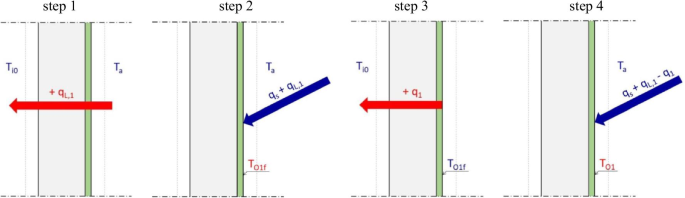

  

  Calculation steps of the one-dimensional model calculations for temperature and heat flow at the building surface—day

Night

A calculation model is implemented which can assess the night-time cooling of buildings. However, in urban areas the night-time heat radiation at ground level is usually very low (Fischer et al. 2008). The dense construction reduces the view to the sky and the façades partially irradiate each other.

The iterative calculation of the surface temperature and the heat flux density between the surface and the surrounding air is carried out analogous to the calculation during the day using the following calculation steps (see Eqs. (12) to (15) and Fig. 7):

• 1. heat conduction—heat flow ${q}_{L,1}$ due to temperature difference, resulting in a decrease of the fictitious homogeneous internal temperature of the monolith:

  $$q_{L,1} = \frac{1}{{R_{T} }}\cdot\left( {T_{a} - T_{i0} } \right).$$

  (12)

• 2. heat radiation and convection—heat flow q_a1 between the heated surface T_O1f and the outside temperature T_a:

  $$q_{a1} = \frac{1}{{R_{{{\text{se}}}} }} \cdot \left( {T_{a} - T_{O1f} } \right) = \frac{1}{{R_{{{\text{se}}}} }} \cdot \left( {T_{a} - T_{O} - q_{L,1} \cdot R_{{{\text{se}}}} } \right).$$

  (13)

${q}_{a1}$ heat flow between the heated outer surface and the outside air in W/m². ${T}_{O}$ initial component surface temperature according to Table 1 in K.

Table 1 Initial temperatures used within the one-dimensional model calculations

• 3. updated heat conduction—fictitious homogeneous internal temperature ${T}_{i1}$:

  $$T_{i1} = T_{i0} + \Delta T = T_{i0} + \frac{{q_{1} \cdot t}}{\chi }.$$

  (14)

• 4. heat flow and actual surface temperature ${T}_{O1}$ at the outer component surface:

  $$T_{O1} = T_{a} + \left( { - 1} \right) \cdot \left( {q_{a1} + q_{1} } \right) \cdot R_{{{\text{se}}}} .$$

  (15)

Fig. 7

Calculation steps of the one-dimensional model calculations for temperature and heat flow at the building surface—night

General boundary conditions

For the one-dimensional model calculations, assumptions are made about the outside temperature, the fictitious inside temperature and the surface temperature at night (see Table 1). The heat transfer resistances are determined depending on the direction of heat flow (see Table 2). The solar heat flux density is assumed to be 500 W/m². With flat roofs, the external heat transfer resistance is assumed to be significantly higher than the standard value because the gravel protects the roof structure from wind. For the calculation of the surface temperatures and heat flows of the ground types, there is no heat transfer resistance inside because the ground has an infinite depth and is not surrounded by a medium. Therefore, only the external heat transfer resistance is considered in the thermal calculations.

Table 2 External and internal heat transfer resistances of the building components and ground surfaces used within the one-dimensional model calculations (Maiullari et al. 2018)

Calculation parameters

In order to be able to assess which building components can be neglected due to the defined error tolerance of 5% for the respective building types, model calculations are carried out on a three-storey apartment building with a gross floor area of 288 m² (floor plan see Fig. 8). The façade is considered to be uniformly painted white with an albedo of 0.7. The average room height of the Gründerzeit building is assumed to be 3.6 m. For the buildings of the 1970s and the new buildings, it is set at 2.6 m.

Fig. 8

Floor plan of all floors of the three-storey apartment building used within the model calculations to assess which building components of the respective building types can be neglected (Natanian et al. 2019)

In the Gründerzeit (from about 1850 to 1914), stairs were made of natural stone, especially limestone or quartz sandstone (Kaiserstein or Rekawinkler stone) (Ahne 2014). Therefore, for the building type Gründerzeit building a Rekawinkler stone is used as staircase material. In the buildings of the 1970s and the new buildings, the calculations are based on stairs in reinforced concrete construction.

The Gründerzeit building and the buildings of the 1970s are calculated with an uninsulated pitched roof with clay roof tiles. The albedo of the red roof skin is 0.225. For the new buildings a flat roof with a gravel covering is considered. The albedo of the flat roof is 0.13 (see Table 3). The internal loads and the heat-storing mass of the facility are neglected.

Table 3 Calculation parameters of the five building types used within the one-dimensional model calculations

The assumptions regarding the albedo of the five ground surfaces are given in Table 4.

Table 4 Assumptions of the albedo of the five ground surfaces used within the one-dimensional model calculations

Simplifications

Based on the calculations carried out on the example building described above, the following components are found to be negligible within the defined error tolerance of 5%:

• 1. neglecting building components due to their mass percentage < 5%

For all types of buildings, the stairs can be neglected when calculating the surface temperature and the heat flow, due to their low mass percentage of the total mass, which is less than 5%.

• 2. neglecting building components when calculating the heat capacity

In new buildings made of reinforced concrete or vertically perforated bricks, the interior components contribute only insignificantly to heat storage. The roof and the outer wall have good thermal insulation properties and minimize the entry of heat into the interior. Table 5 shows the types of buildings for which the contribution of the interior components to heat storage can be neglected.

Table 5 Relevance of the interior components with regard to heat storage according to the results of the one-dimensional model calculations

Sensitivity analysis

The three parameters—albedo, area-related effective heat capacity and thermal resistance—have a significant influence on the surface and interior temperature of building and ground types. In order to be able to determine this influence, the parameters are varied within the one-dimensional simulations, which are run for two time steps in Microsoft Excel. For each parameter and building or ground type three values are used for the sensitivity analysis: the actual value, a reduced value (50%) and an increased value (150%). Subsequently, trends of the fictitious indoor or surface temperature depending on the three parameters are generated. This can be used to determine how sensitive a type is to a parameter.

In terms of the fictitious indoor temperature, building type G4 (new concrete building) is the least sensitive to a change in all three parameters. Building type G3 (1970s brick building) is the most sensitive to a change in heat capacity of the exterior wall, whereas building type G2 (1970s concrete building) is the most sensitive to a change in albedo and thermal resistance. In the case of ground surfaces, type B3 (paved road) is the least sensitive. Contrarily, ground type B5 (meadow) is the most sensitive to a change in thermal resistance and ground type B1 (asphalt road) is the most sensitive to a change in albedo as well as heat capacity.

In the case of the exterior roof components, a relationship can be established between the absolute value and the sensitivity: the greater the heat capacity, the lower is the sensitivity to a change. This statement is also valid for the thermal resistance of the roof components. For the exterior wall constructions, though, there is no correlation noticeable. With increasing heat capacity, the sensitivity of the fictitious interior temperature to a change in the three parameters decreases. In general, the sensitivity of the fictitious internal temperature of the building and ground monoliths is greatest to a change in thermal resistance, then to a change in albedo and least to a change in heat capacity.

In order to validate the uhiSolver software after implementation of the gained knowledge on the basis of a real object, in part two of this research work (see Sect. “Validation case Kandlgasse”), the simulation results of a residential block in Vienna are compared with measurement data collected on site.

Validation case Kandlgasse

The aim of the implementation of the simplified material data for the five most common types of building volumes and ground surfaces in the simulation software uhiSolver is to verify the forecast quality of the applied model, i.e., the sensitivity of the simulated air temperature with respect to the averaging of heat capacity, heat conduction and specific density (c_p, λ, ρ). The physical boundary conditions (initial temperatures and heat transfer resistances) as well as the surface properties (albedo) listed in the first part of this research work (see Sect. “Generation of simplified material data”) are also incorporated into the model parameters.

Simulation setting

Within the framework of the research project “GrünPlusSchule” (Korjenic 2018), funded by the FTI initiative Stadt der Zukunft 2nd call for proposals, a measurement campaign was carried out between May 2015 and May 2018 at the school GRG 7 Kandlgasse in Vienna, which was intended to investigate the effect of façade greening on outside and inside temperatures as well as heat flows within the masonry. As shown in Fig. 9, different greening measures were applied within the inner courtyard and on top of the roof of the school’s gymnasium. The measurement data collected on site were air temperature and relative humidity behind (ventilation gap) and in front of the façade greening as well as on the greened roof. The instruments used to measure air temperatures were Lin Piccos A05. They were fitted with a radiation shield. Measurements were taken at 5- to 10-min intervals over the entire project period. The data collected in summer 2017 are used to validate uhiSolver and are compared with the simulation results.

Fig. 9

Greening systems (red lines) and measurement positions (blue dots) within the inner courtyard at the school GRG 7 Kandlgasse in Vienna

The date of the simulation is August 1, 2017, a cloudless hot day with inner-city temperatures of 35 °C, which were also measured in Kandlgasse in the afternoon.

Numerical details

Temporal coupling between heat conduction in building envelopes and CFD is performed as full two-way coupling with methods and algorithms also used in chtMultiRegionFoam, a conjugate heat transfer solver included in OpenFOAM. A modified solar calculator library is implemented in OpenFOAM. Heat conduction iteration and coupling is 1:1 in the solver; heat conduction is solved every time step. Radiation (due to high computational demand) is solved every n fluid iterations. Sun position is updated every 10 min of the simulated time. Radiation model is multi-band and active throughout the simulation, under “day” (sun elevation angle > 0°) and “night” (sun elevation angle < 0°, solar radiation off) conditions.

In addition to the interaction of radiation and air with the buildings, existing plants (green walls, trees) are fully included in the simulation with all their thermodynamic effects: reflection, shadows and evapotranspiration. In the current version of uhiSolver all vegetation zones are treated the same:

• Evapotranspiration rate is modulated by local radiation density and dry bulb temperature and limited by local relative humidity (driving force) and local wind-speed (transport limitation).

• Appropriate sink terms are used for radiation (optical absorption and emission coefficients) and momentum (via porosity terms).

• Any substrate material not in direct contact with a building is not considered in the current version.

Within the vegetation model in uhiSolver transpiration of plants is taken into account as follows:

• Local water vapor pressure and water vapor saturation pressure is calculated using Antoine equation.

• Local dew point and saturation loading are derived from Antoine equation.

• Zero evapotranspiration rate is reached if local conditions are saturated (100% RH).

• Max evapotranspiration rate is reached if local RH is very low and local evapotranspiration modulator (due to temperature and radiation) is very high.

• Specific leaf density goes into Darcy–Forchheimer coefficients of porous zone of finite volume cells designating vegetation and also into absorption/emission coefficients for solar radiation damping (shading) of said volume zones.

• Heat for evapotranspiration (modulated and limited by above parameters) is taken directly out of fluid finite volume cell (taking into account thermodynamic gas mixture properties).

• Local state is updated immediately; temperature, saturation, loading, density and solver advances to next module and solves for dynamic pressure and velocity in next time-step.

The used simulation models, discretization algorithms and matrix solver settings for the fluid phase (air) are:

• Compressible, buoyant, unsteady simulation with forcing of log profile in-flow of wind-speed, time-varying and height constant humidity loading, time-varying and height constant temperature and time-varying incoming solar radiation vector and intensity

• Turbulence model is k-epsilon based with modified model constants suitable to achieve horizontal wind profile stability for applications of atmospheric boundary layer flows

• Pressure–velocity coupling using the PIMPLE algorithm for stabilization of local conditions, which can cause the CFL number to be greater than one temporarily

• Adaptive time stepping to keep maximum CFL number constant in fluid domain

• Temporal (backwards differencing) and spatial (upwind differencing of fluxes) discretization having 2nd order accuracy

• Central differencing (with corrections) is used for gradient calculations and Laplacian based schemes

• Solution of density field using Pre-conditioned Conjugate Gradient solver with solution tolerance of 1e–7

• Solution of discretized radiation directions (via fvDOM model) using Generalized Algebraic Multigrid solver with symmetric Gauss–Seidel smoother with solution tolerance 1e–4

• Solution of other variables using Pre-conditioned Bi-conjugate gradient solver with stabilization and solution tolerance 1e–7

• Pressure–velocity coupling is active for all time steps and no frozen flux approach is employed to keep solution coupling tight.

The used simulation models, discretization algorithms and matrix solver settings for solid phases (building volumes and ground) are:

• Time discretization: forward Euler

• Interpolation: central differencing, Laplacian schemes: central differencing using correction.

For further information, some basic equations and their implementation in uhiSolver are included in the supplementary material (Additional file 1: Appendix C).

The simulation approach of uhiSolver shall be scaled from single city-block (as shown in this publication) to neighborhood level (10 blocks, ongoing research). Dealing with more blocks necessitates a simplified geometry and boundary condition work-flow and automation procedures to enable effective microclimate simulations and affordable parameter studies as the labor costs for manual program interactions significantly outweigh computational costs. The presented results are the first steps in this direction.

Simulation results

The results of the uhiSolver simulation for the selected day are shown as temperature profiles over the first 24 h of the simulation for nine different positions within the inner courtyard. Measurement data are available for only one position and are compared with the simulation results (detailed information on the experimental and simulation data is provided in the Additional file 1: Appendix D. Subsequently, 2D and 3D renderings of the apparent temperature, air temperature, air flow velocity, relative humidity, radiation density and incident surface radiation of the courtyard and its surroundings are presented for the hottest time of the day (14:00 CEST).

The selected positions (probe 01 to probe 09) are given in Fig. 10. The temperature profiles (radiation protected, i.e., shaded temperature) of each position are superimposed in Fig. 11, showing the temperatures with and without evapotranspiration compared to the forced inlet temperature. The impact of evapotranspiration on the simulated temperatures is almost negligible, as can be seen in Fig. 12 (giving the simulation results for probe 01 behind the south oriented façade greening), and decreases rapidly with increasing distance from the façade greenery. The temporarily slightly increased temperatures in the simulation with evapotranspiration is explained by minimally changed flow conditions due to buoyancy and density differences because of evaporation and mixing of air from warmer layers.

Fig. 10

Selected positions for the evaluation of the simulated temperature profiles within the transient simulation with uhiSolver

Fig. 11

Overview of the temperature profiles of probes 01–09 with (green lines) and without evapotranspiration (grey lines) compared to the forced inlet temperature (red line)

Fig. 12

Temperature profiles of probe 01 with (green line) and without evapotranspiration (grey line) compared to the forced inlet temperature (red line)

A comparison of the measured data of air and surface temperatures with the simulation results shows a good accordance. With respect to the air temperature in the area of the façade greening, the deviation between measured data and simulation results is small, especially in the afternoon and evening hours. The absolute error between measurement data and simulation results is within ± 2 Kelvin for the validation case (see Figs. 13 and 14). The largest deviations occur in the morning hours between 7 and 9 o’clock as well as after 6 o’clock in the evening. The reason for this is homogenous initialization of building temperatures and over-simplification of evapotranspiration kinetics, with evapotranspiration rates (mm/day) being calculated based on measurement data from 2017 available for the monthly average water use of the façade greening system “Techmetall”. This is a field of active code development and research and future versions of uhiSolver will improve accuracy in that regard.

Fig. 13

Comparison of simulation results with evapotranspiration (green line) and measurement data (blue dots) for the validation case Kandlgasse compared to the forced inlet temperature (red line)

Fig. 14

Absolute error between simulation results with evapotranspiration (green line) and measurement data (violet crosses) for the validation case Kandlgasse

The evaluation of the simulation results clearly shows that the apparent temperature (Steadman 1994) in the greened inner courtyard is comparable to that of the adjacent streets and in some cases even higher (see Fig. 15). However, the air temperature, measured in the shadow and without the influence of radiation, is 2 °C below that of the surrounding area (see Fig. 16), which is due to the cooling capacity of the plants and the lower albedo. The reasons for this are:

• lower air flow velocities in the inner courtyard (hardly any wind and therefore hardly any moisture removal, see Fig. 17),

• higher relative humidity in the inner courtyard compared to the surrounding streets due to the evapotranspiration of the plants (see Fig. 18) and

• ‘spandrels’ in the inner courtyard with direct radiation and additionally reflected secondary radiation of the walls (see Fig. 19).

Fig. 15

Apparent temperature (Steadman 1994) of the simulation case Kandlgasse, 1.5 m above the ground at 14:00 CEST on 01 August 2017

Fig. 16

Air temperature (dry bulb temperature) of the simulation case Kandlgasse, 1.5 m above the ground at 14:00 CEST on 01 August 2017

Fig. 17

Velocity of air flow of the simulation case Kandlgasse, 1.5 m above the ground at 14:00 CEST on 01 August 2017

Fig. 18

Relative humidity of the simulation case Kandlgasse, 1.5 m above the ground at 14:00 CEST on 01 August 2017

Fig. 19

Radiation density of the simulation case Kandlgasse, 1.5 m above the ground at 14:00 CEST on 01 August 2017, shown as spherical integral over all spatial directions

Representative instantaneous fields were chosen at the apex of urban heat after midday (at 14:00 CEST). For better understanding, the above mentioned illustrations (Figs. 15, 16, 17, 18, 19) are shown as 2D section and 3D rendering at the same time.

The incident radiation (W/m²) on the surfaces is shown as a blackbody color scheme in Fig. 20 to illustrate the hot ‘spandrels’ with IR reflections. It is noticeable that the highest radiation intensities occur in the corners of the inner courtyard. These are also exactly those areas where the maximum values of the apparent temperature are to be expected.

Fig. 20

Incident surface radiation (W/m²) of the simulation case Kandlgasse at 14:00 CEST on 01 August 2017

Discussion

For a better understanding of the validity of the above presented simulation results, they are compared to similar studies. In a study of Antoniou et al. (2019) CFD simulations of urban microclimate are performed for a dense highly heterogeneous district in Nicosia, Cyprus and validated using a high-resolution dataset of on-site measurements of air temperature, wind speed and surface temperature conducted for the same district area. The CFD simulations are performed based on the 3D Unsteady Reynolds-Averaged Navier–Stokes (URANS) equations and the simulated period covers four consecutive days in July 2010. It is shown that the CFD simulations can predict air temperatures with an average absolute difference of 1.35 °C, wind speed with an average absolute difference of 0.57 m/s and surface temperatures with an average absolute difference of 2.31 °C.

A case study of Maiullari et al. (2018) uses a coupling approach that links the simulation tools ENVI-met and City Energy Analyst. The comparison of the air temperature from the weather station and average air temperature from ENVI-met around the buildings of an urban re-development project in the city of Zurich, Switzerland, shows a maximum deviation of 2.5 °C mainly during the night for a cool day and of 3 °C at 11 o’clock in the morning for a hot day.

Another study of Natanian et al. (2019) couples ENVI-met and EnergyPlus to bring together energy and microclimatic modeling for a synergetic assessment at the block scale in the climatic context of Tel Aviv. A comparison of the daily resultant air temperature recorded for three different weather files (EnergyPlus, Urban Weather Generator (UWG) and ENVI-met) for the 26th of July recorded for the highest density scenario for three different typologies (courtyard, scatter and high-rise) shows a night-time air temperature increase of up to 1.5 °C within the UWG file compared to the rural EnergyPlus file. The ENVI-met file recorded a higher night-time temperature increase of up to 3 °C but also a day-time temperature drop of up to 1.5 °C.

In a work of Diz-Mellado et al. (2021) the applicability of a supervised Machine Learning (ML) model as a suitable tool for predicting microclimatic performance inside courtyards has been evaluated. For this purpose, among the ML models developed as supervised learning, Support Vector Machines were selected. The final results for two selected validation cases located in the South of Spain showed that, when the day-time slot with the highest urban overheating is considered, the relative error is almost below 0.05% and the Root Mean Square Error (RMSE) is around 1 °C.

Compared to the studies mentioned above, good results (equal to or better than established methods) are obtained with an absolute error between measurement and simulation of ± 2 °C for the validation case Kandlgasse presented in this work, despite the simplifications proposed. Another validation case in the area of Gablenzgasse in Vienna is currently in progress—first simulation results are included in the Additional file 1: Appendix E.

While in the validation case Kandlgasse the sensors were placed relatively close to each other (a few meters) and their transient response was monitored, the validation case Gablenzgasse used distributed measurement locations (spaced tens to hundreds of meters apart) at different fixed points in time. Employing a statistical analysis of the two validation cases, the transient response quality (how well does the simulation result follow measured values) and the spatial response quality (how well does the simulation result fit at different locations) of uhiSolver can be separated from each other. Statistical results and raw data of both validation cases are included in the Additional file 1: Appendix D.

Statistical analysis of correlation coefficients and standard deviations of temperatures shows:

• The transient validation case Kandlgasse is highly correlated to measurement data. Within a 24-h period the standard deviation of temperature differences (simulated to measured) is 0.99 °C.

• The spatially distributed validation case Gablenzgasse shows low deviations of simulated temperatures compared to measured temperatures. The standard deviation of temperature differences (simulated to measured) is 0.93 °C.

• Spatial and temporal standard deviations of temperature differences are both below 1.00 °C.

• uhiSolver shows relatively high spatial and temporal accuracy for temperature predictions. Absolute accuracy (defined via standard deviation) is within 1.00 °C for both validation cases. Relative thermal accuracy is in the range of 10% for hot, cloudless days when compared to a daily thermal variation of 10 °C. 10% accuracy is often considered to be sufficient when used as an engineering tool in the design phase.

More detailed field measurements will be conducted as part of another research program to provide sufficient data for the next validation study. However, further validation of the uhiSolver software also by comparing the simulation results with those of other microclimate simulation tools is needed to substantiate the accuracy of this model using simplified material data for building components and ground surfaces.

Conclusions

The five most relevant building types and ground surfaces in Vienna are investigated. By means of error weighting and sensitivity analysis, it is determined which parameters are essential in each case and which can be neglected. Finally, the defined building types and ground surfaces are reduced in their inhomogeneous material properties to such an extent that they can be represented as a homogeneous monolith with a known margin of error in the computer model.

Considering the defined error tolerance of 5%, it does appear that the stairs can be neglected in all building types due to their low mass share in the total mass. The doors can also be neglected in the mass determination of the interior walls. However, the influence of window surfaces on the surface and interior temperature is significant, since the windows, taking into account shading devices, lead to a reduction in the overall albedo compared to a purely white façade. This results in a higher heat absorption and thus a higher total heat input.

Taking the defined boundary conditions into account, one-dimensional model calculations are carried out for only two time steps in order to derive a tendency for the different parameters and relationships (this forms the algorithmic basis for the transient simulations presented in part two). It is shown that the surface temperatures are related to numerous factors, since the mutual dependence (irradiation and radiation as well as heat conduction and storage) is complex. Therefore, more accurate forecasts can only be made with dynamic calculations (as in uhiSolver), taking into account a complete physical coupling of all effects: heat conduction, radiation, solar path, airflow and evaporation.

The Dynamic 3D simulations carried out in part two of this study confirm that the simplifying assumption of homogeneous material data for building bodies provides very good results for the investigated validation case of the school GRG 7 Kandlgasse in Vienna.

The simulations carried out also show that the apparent temperature in the greened inner courtyard of the school is sometimes perceived higher than in the adjacent streets, despite the lower air temperature. The reasons for this are the higher radiation density due to the mutual irradiation of the courtyard façades, the lower air velocities and the higher air humidity compared to conditions outside the courtyard.

In the coming years, the demand for a tool that can significantly reduce the extent of the influence of urban structure, the building materials used and the surfaces on urban heat islands in the planning phase will steadily increase. The reasons for this are increasing urbanization and global warming. The simulation software uhiSolver is such a planning tool and is able to help understand the interaction between urban microclimates and the buildings.

References

Ahne V (2014) Alte Steinstiegen auf dem Prüfstand. Die Presse, Wien
Ansys. https://www.ansys.com/
Antoniou N, Montazeri H, Neophytou M, Blocken B (2019) CFD simulation of urban microclimate: validation using high-resolution field measurements. Sci Total Environ 695:133743. https://doi.org/10.1016/j.scitotenv.2019.133743
Ausführungsplan (2015) Wien: atelier kaindl + kuntner gmbh
Austrian Standards Institute (2008) “ÖNORM EN ISO 13786: thermal performance of building components—dynamic thermal characteristics—calculation methods
B. of M. Commonwealth of Australia (2010) Thermal Comfort observations. http://www.bom.gov.au/info/thermal_stress/ (accessed Sep. 03, 2020)
Baumgartner CM (2019) Influence of different construction methods and soil types on the Urban Heat Island-Effect. Vienna University of Technology
Cid K, Vianna S (2016) A comparative study between thermal radiation models P-1 and discrete ordinates using Cfd software openfoam. In: Congresso Brasileiro de Fluidodinâmica Computacional, I: 1–5. https://doi.org/10.17648/cbcfd-44247
Clauser C (2014) Einführung in die Geophysik—Globale physikalische Felder und Prozesse in der Erde. Springer Spektrum, Berlin
Coelho PJ, GonÇalves JM, Carvalho MG, Trivic DN (1998) Modelling of radiative heat transfer in enclosures with obstacles. Int J Heat Mass Transf 41(4–5):745–756. https://doi.org/10.1016/S0017-9310(97)00158-0
Diz-Mellado E, Rubino S, Fern S, Macarena G (2021) Applied machine learning algorithms for courtyards thermal patterns accurate prediction. Mathematics 9(10):1142. https://doi.org/10.3390/math9101142
ENVI_MET Decoding urban nature. https://www.envi-met.com/de/
ENVI-met Model Architecture (2019). http://envi-met.info/ (accessed Sep. 23, 2020)
FFG IS5k, Final report, Nr. 849231, project ‘vmSol’, Rheologic GmbH and TU Vienna, 20.10.2015, internal communication
Fischer M, Heinz-Martin F, Hanns H, Peter H, Martin J, Richard R, Ekkehard S (2008) Lehrbuch der Bauphysik, 6th edn. Vieweg Teubner Verlag GWV Fachverlage GmbH, Wiesbaden
Gameiro da Silva MC (2013) Spreadsheets for the calculation of thermal comfort indices. Scribd. https://doi.org/10.1073/pnas.1017993108
GREENPASS Software. https://greenpass.io/software/
Hollands J, Tudiwer D, Korjenic A, Bretschneider BB (2018) Greening Aspang—Messtechnische Untersuchungen zur ganzheitlichen Betrachtung mikroklimatischer Wechselwirkungen in einem Straßenzug einer urbanen Hitzeinsel. Bauphysik 40(3):105–119. https://doi.org/10.1002/bapi.201810014
Holopainen R (2012) A human thermal model for improved thermal comfort. Doctor of Science in Technology Thesis, Aalto University, VTT
Honjo T (2009) Thermal comfort in outdoor environment. Glob Environ Res 13:43–47
Huttner S, Bruse M (2009) Numerical modeling of the urban climate—a preview on ENVI-MET 4.0. Seventh Int Conf Urban Clim 4
Ismail KAR, Salinas CT (2004) Accurate computing of radiative source term using discrete ordinates methods for to use in CFD codes. Conference: Fourth European Thermal Sciences 1:110–119
Jendritzky G, Maarouf A, Staiger H (2001) Looking for a universal thermal climate index UTCI for outdoor applications. Paper presented at the Windsor-Conference on Thermal Standards
Knaus H, Schneider R, Han X, Strohle J, Schnell U, Hein KRG (1999) Comparison of different radiative heat transfer models and their applicability to coal-fired utility boiler simulations. 4th International Conference on Technologies and Combustion for a Clean Environment. http://elib.uni-stuttgart.de/opus/volltexte/1999/277/
Korjenic A, et al (2018) GrünPlusSchule@Ballungszentrum Hocheffiziente Fassaden- und Dachbegrünung mit Photovoltaik Kombination; optimale Lösung für die Energieeffizienz in gesamtökologischer Betrachtung. Endbericht, Stadt der Zukunft, FFG/BMVIT, Wien
Korjenic A, et al (2020) GRÜNEzukunftSCHULEN - Grüne Schuloasen im Neubau. Fokus Planungsprozess und Bestandsgebäude. Endbericht; FFG; Wien
Maiullari D, Mosteiro-Romero M, Pijpers-Van Esch M (2018) Urban microclimate and energy performance: an integrated simulation method. 34th International Conference on Passive and Low Energy Architecture (PLEA) - Smart Healthy Within the Two-Degree Limit 1:384–389
Mitterböck M, Korjenic A (2017) Analysis for improving the passive cooling of building’s surroundings through the creation of green spaces in the urban built-up area. Energy Build 148:166–181
Mould ST (2019) The solarLoad Radiation Model. dtx-colab.pt
Mu D, Gao N, Zhu T (2018) CFD investigation on the effects of wind and thermal wall-flow on pollutant transmission in a high-rise building. Build Environ 137:185–197
Mursch-Radlgruber E, Trimmel H, Gerersdorfer T (2009) Räumliche Differenzierung der mikroklimatischen Eigenschaften von Wiener Stadtstrukturen und Anpassungsmaßnahmen. Ergebnisse kleinklimatischer Messungen. Teil 2 der Studie Räumlich und zeitlich hoch aufgelöste Temperaturszenarien für Wien und ausgewählte. Wiener Umweltschutzabteilung (MA 22), EU-Strategie und Wirtschaftsentwicklung (MA 27)
Natanian J, Maiullari D, Yezioro A, Auer T (2019) Synergetic urban microclimate and energy simulation parametric workflow. J Phys Conf Ser 1343:012006. https://doi.org/10.1088/1742-6596/1343/1/012006
Pecka A (2014) Finite Volume Method for Radiative Heat Transfer Problems. University of West Bohemia
Sá da Costa PP (2016) Validation of a mathematical model for the simulation of loss of coolant accidents in nuclear power plants. Técnico Lisboa
Schmid E, Pröll T (2020) Umwelt- und Bioressourcenmanagement für eine nachhaltige Zukunftsgestaltung. Springer Spektrum, Berlin
Steadman RG (1994) Norms of apparent temperature in Australia. Aust Met Mag 43:1–16
Technische Universität Wien and Universität für Bodenkultur Wien (2018) Forschungsbericht Vegetationstechnisches und bauphysikalisches Monitoring des ‘Vertikalen Gartens’ der MA31 in der Grabnergasse 4-6, 1060 Wien. Wien
Terjung WH, O’Rourke PA (1980) Simulating the causal elements of urban heat islands. Boundary-Layer Meteorol 19(1):93–118. https://doi.org/10.1007/BF00120313
Toparlar Y, Blocken B, Vos P, van Heijst GJF, Janssen WD, van Hooff T, Montazeri H, Timmermans HJP (2015) CFD simulation and validation of urban microclimate: a case study for Bergpolder Zuid, Rotterdam. Build Environ 83:79–90. https://doi.org/10.1016/j.buildenv.2014.08.004
Toparlar Y, Blocken B, Maiheu B, van Heijst GJF (2017) A review on the CFD analysis of urban microclimate. Renew Sustain Energy Rev 80:1613–1640. https://doi.org/10.1016/j.rser.2017.05.248
United Nations Department of Economic and Social Affairs (2019) World Urbanization Prospects 2018: Highlights. https://population.un.org/wup/
Urban Weather Generator 4.1 urban heat island effect modeling software. http://urbanmicroclimate.scripts.mit.edu/uwg.php
Zentralanstalt für Meteorologie und Geodynamik (2002) Klimadaten von Österreich 1971–2000. http://www.zamg.ac.at/fix/klima/oe71-00/klima2000/klimadaten_oesterreich_1971_frame1.htm (accessed Aug. 07, 2020)
Acknowledgements
This research was supported by the Austrian Research Promotion Agency (FFG) within the framework of the General Programme funding line as well as by the Federal Ministry for Climate Action, Environment, Energy, Mobility, Innovation and Technology (BMK) within the Cities of the Future funding line.
Funding
This research was funded by Österreichische Forschungsförderungsgesellschaft FFG—feasibility study, Grant number 873045.
Author information
Authors and Affiliations
Contributions
FT: conceptualization, writing—original draft preparation, project administration. CMB: methodology, investigation, resources, data curation, visualization. AH and ML: software, validation, visualization, funding acquisition. AK: formal analysis, writing—review and editing, supervision. All authors read and approved the final manuscript.
Corresponding author
Ethics declarations
Ethics approval and consent to participate
Not applicable.
Consent for publication
Competing interests
The authors declare that they have no competing interests.
Additional information
Publisher's Note
Springer Nature remains neutral with regard to jurisdictional claims in published maps and institutional affiliations.
Supplementary Information
Additional file 1.
Appendix.
Rights and permissions
Open Access This article is licensed under a Creative Commons Attribution 4.0 International License, which permits use, sharing, adaptation, distribution and reproduction in any medium or format, as long as you give appropriate credit to the original author(s) and the source, provide a link to the Creative Commons licence, and indicate if changes were made. The images or other third party material in this article are included in the article's Creative Commons licence, unless indicated otherwise in a credit line to the material. If material is not included in the article's Creative Commons licence and your intended use is not permitted by statutory regulation or exceeds the permitted use, you will need to obtain permission directly from the copyright holder. To view a copy of this licence, visit http://creativecommons.org/licenses/by/4.0/.
About this article
Cite this article
Teichmann, F., Baumgartner, C.M., Horvath, A. et al. Simulation of urban microclimate with uhiSolver: software validation using simplified material data. Ecol Process 10, 67 (2021). https://doi.org/10.1186/s13717-021-00336-y
Received:
Accepted:
Published:
DOI: https://doi.org/10.1186/s13717-021-00336-y